The Challenge
“I believe that we are just at the beginning of the Earth Observation big data revolution. Joint effort and open science are the fundamental bricks to build new models and services for addressing societal challenges.” Dr. Andrea Nascetti, Faculty of Sciences, University of Liège
Motivation
Forests are adding and removing carbon dioxide from the air all the time. How do we know how much? The answer lies in aboveground biomass (AGBM), a widespread measure in the study of carbon release and sequestration by forests. Current approaches to measuring biomass, range from destructive sampling, which involves cutting down a representative sample of trees and measuring attributes such as the height and width of their crowns and trunks, to remote sensing methods. Remote sensing methods offer a much faster, less destructive, and more geographically expansive biomass estimate.
In our BioMassters challenge, competitors used satellite imagery of Finnish forests from Sentinel-1 and Sentinel-2, earth observation satellites developed by the European Commission and the European Space Agency as a part of the Copernicus program. The ground truth for this competition came from LiDAR (Light Detection And Ranging) and in-situ measurements of the same forests collected by the Finnish Forest Centre on an annual basis.
The goal of the BioMassters challenge was to estimate the yearly biomass of 2,560 meter by 2,560 meter patches of land in Finland's forests using S-1 and S-2 imagery of the same areas on a monthly basis. Let's see how the winners of this challenge bio-passed the test!

Sentinel-1. Image credit: ESA Sentinel Online |

Sentinel-2. Image credit: ESA Sentinel Online |
Results
Over the course of the competition, participants tested over 1,000 solutions and were able to contribute powerful models to the estimation of AGBM using satellite images. To kick off the competition, Mathworks, the competition's sponsor, released a benchmark solution that demonstrated how to make predictions using a simple UNet model.
The metric for this competition was Average Root Mean Square Error (RMSE), where RMSE was calculated for each image, and then averaged over all images in the test set. This is an error metric, so a lower value is better.
The participants were able to achieve impressive results, with the top-scoring finalist achieving an Average RMSE of 27.63, the second-place winner scoring 27.68, and the third-place winner scoring 28.04. These scores represent not only a substantial improvement over the benchmark model (which had a score of 101.98), but great promise for exceeding some of the most widely available open-source biomass measurements available.
One of the largest biomass estimation projects, the ESA biomass CCI project provides global maps at 100-meter spatial resolution, while participants provided maps at 10-meter resolution. Traditional biomass estimates, including those used in the CCI project, use only traditional remote sensing modeling approaches that do not integrate multi-modal data (such as the data collected by S-2 that participants used in this challenge) and are at lower temporal resolutions.
To build these high-performing models, the winners brought a wide variety of creative strategies to this task! Below are a few interesting approaches:
- Feature engineering: Participants were given monthly images each from S-1 and S-2 to estimate yearly biomass. The first and third place winner chose to aggregate these monthly images rather than using a time-series approach. The first place winner used self-attention to aggregate over all 12 months, and the third place winner reduced the number of images per plot to 6 using median composites. The second place winners used a time-series approach by treating time as a third dimension and passing the 3-D features they created into a 3-D image segmentation model.
- Image augmentations: As is standard in many computer vision tasks, all three finalists used augmentation of the training images, including flips and rotations.
- Model architectures: All three finalists used some variation of a UNet architecture, which is among the most popular for computer vision tasks. The first place winner used a standard UNet CNN, while the third-place winner used a UNet++ model. The SWIN UNETR (UNet TRansformers) model used by the second place winners is also a type of UNet model adapted for 3-D MRI.
Now, let's get to know our winners and how they created such successful biomass estimation models! You can also dive into their open source solutions in the competition winners' repo.
Meet the winners
| Prize | Name |
|---|---|
| 1st place | kbrodt |
| 2nd place | Team Just4Fun |
| 3rd place | yurithefury |
| MATLAB Bonus | Team D_R_A_K |
Kirill Brodt

Place: 1st Place
Prize: $5,000
Hometown: Almaty, Kazakhstan
Username: kbrodt
Background:
I'm doing research at the University of Montréal in computer graphics. I got my master's in mathematics at the Novosibirsk State University, Russia. I am involved in an educational program where I teach machine and deep learning courses. I am a research supervisor of undergraduate students and bachelors’ theses.
What motivated you to compete in this challenge?
Machine learning is my passion and I often take part in competitions.
Summary of approach:
The solution is based on an UNet model with a shared encoder with aggregation via attention. The inputs to the encoder are 15-band images with a resolution of 256x256 from joint Sentinel-1 and Sentinel-2 satellite missions. The encoder is shared for all 12 months. The outputs are aggregated via self-attention. Finally, a decoder takes as inputs the aggregated features and predicts a single yearly agbm. Optimization was performed using AdamW optimizer and CosineAnnelingLR scheduler and RMSE loss. We don't compute loss for high agbm values (>400). We use vertical flips, rotations, and random month dropout as augmentations. Month dropout simply removes images.
What are some other things you tried that didn’t necessarily make it into the final workflow?
I tried 3D CNNs, segformer models, aggregation level on different levels (before encoder, after encoder, after decoder), different attention models, group norm.
If you were to continue working on this problem for the next year, what methods or techniques might you try in order to build on your work so far?
Make predictions non-negative, i.e. put relu layer on top logits.
Team Just4Fun

Qixun Qu |

Hongwei Fan |
Place: 2nd Place
Prize: $2,000
Hometown: Chengdu, Sichuan, China (Qixun Qu) and Nanjing Jiangsu, China (Hongwei Fan)
Username: qqggg, HongweiFan
Background:
I (qqggg, Qixun Qu in real name) am a vision algorithm developer and focus on image and signal analysis.
I (Hongwei Fan) am a PhD student affiliated with the Data Science Institute, Imperial College London. Before my PhD, I completed a Masters degree in biomedical engineering at Tsinghua University and worked as an algorithm engineer at SenseTime.
What motivated you to compete in this challenge?
As our team name Just4Fun, we are excited to solve more interesting problems than what we did at work to have fun.
Summary of approach:
We defined this task as a temporal-spatial regression problem. Thus, we applied a 3D neural network to make regression.
- S1 and S2 features and AGBM labels were carefully preprocessed according to statistics of training data. Outliers were replaced by the lower or upper limitations.
- Training data was splited into 5 folds for cross validation.
- Processed S1 and S2 features were concatenated to 3D tensor in shape [B, 15, 12, 256, 256] as input, targets were AGBM labels in shape [B, 1, 256, 256].
- Some operations, including horizontal flipping, vertical flipping and random rotation in 90 degrees, were used as data augmentation on 3D features [12, 256, 256] and 2D labels [256, 256].
- We applied Swin UNETR with the attention from Swin Transformer V2 as the regression model. Swin UNETR was adapted from the implementation by the MONAI project.
- In training steps, Swin UNETR was optimized by the sum of weighted MAE and SSIM Loss. RMSE of validation data was used to select the best model.
- We trained Swin UNETR using 5 folds, and got 5 models.
- For each testing sample, the average of 5 predictions was the final result.
What are some other things you tried that didn’t necessarily make it into the final workflow?
- We tried to add focal frequency loss as a regression constraint to optimize Swin UNETR. But it didn’t improve the evaluation metric.
- We tried to train VT-Unet but got much worse results on local cv. VT-Unet is also a 3D UNet-like semantice segmentation model, whose both enconder and decoder are Swin Transformer.
If you were to continue working on this problem for the next year, what methods or techniques might you try in order to build on your work so far?
First of all, we will reimplement the statistics calculation using a two-pass method, to extremely reduce the memory usage. Our current approach has the potential to improve if we tuned hyper-parameters more carefully. We will try some other 3D transformer based regression models, and try to apply some self-supervised techs to get pre-trained models.
Yuri Shendryk

Place: 3rd Place
Prize: $1,000
Hometown: Sydney, Australia
Username: yurithefury
Background:
I am a Geospatial Data Scientist at Dendra Systems. Here I develop algorithms to process terabytes of satellite and airborne data – work that enables Dendra Systems to monitor and restore complex and biodiverse ecosystems. Prior to Dendra, I spent multiple years studying and working in the field of Geoinformatics in Ukraine, Sweden, and Germany, after which I earned my PhD degree in Geography at UNSW in Australia. Currently, my work is centered around the integration of Remote Sensing and Machine Learning for monitoring reforestation and ecological restoration projects.
What motivated you to compete in this challenge?
As the first DrivenData competition I have participated in, I was drawn to the BioMassters challenge because of the importance of its mission. Forests play a critical role in removing carbon dioxide from the atmosphere and storing it as biomass. The BioMassters challenge is one of the global community’s efforts to protect and restore forests, and I wanted to be part of the solution. Hopefully, my work will bring us a step closer to knowing how much carbon is being sequestered by forests and monitoring change over time, and to the ultimate goal of ensuring accountability and building community confidence in the value of carbon sequestration projects. I also wanted to see how my machine learning skills stack up against the best in the field.
Summary of approach:
- Sentinel-1 and Sentinel-2 imagery were preprocessed into 6 cloud-free median composites to reduce data dimensionality while preserving the maximum amount of information
- 15 models were trained using a UNet++ architecture in combination with various encoders (e.g. se_resnext50_32x4d and efficientnet-b{7,8}) and median cloud-free composites. From the experiments, UNet++ showed better performance as compared to other decoders (e.g UNet, MANet etc.)
- The models were pretrained with multiple augmentations (HorizontalFlip, VerticalFlip, RandomRotate90, Transpose, ShiftScaleRotate), batch size of 32, AdamW optimizer with 0.001 initial learning rate, weight decay of 0.0001, and a ReduceLROnPlateau scheduler
- UNet++ models were optimized using a Huber loss to reduce the effect of outliers in the data for 200 epochs
- To improve the performance of each UNet++ model they were further fine-tuned after freezing pre-trained encoder weights for another 100 epochs
- For each model the average of 2 best predictions was used for further ensembling
- The ensemble of all 15 models using weighted average was used for the final submission
What are some other things you tried that didn’t necessarily make it into the final workflow?
- MSE loss on logarithmic and sqrt scaled agb data
- Model ensembling using LightGBM
- Model stacking using a CNN-based meta learner
- Adding vegetation indices for Sentinel-2 and VV/VH ratio for Sentinel-1 images
- TweedieLoss and RMSLELoss
If you were to continue working on this problem for the next year, what methods or techniques might you try in order to build on your work so far?
- Incorporating time and location information for each pixel (i.e. latitude and longitude)
- Incorporating elevation and land cover information
- Continue experimenting with other loss functions
- Cross-validation
- Potentially better architectures (e.g. UNet3+ or Transformers)
- Getting more GPUs for hyperparameter tuning and faster training/inference
Team D_R_K_A
Azin Al Kajbaf |
Kaveh Faraji |
Place: MATLAB Bonus Prize
Prize: $2,000
Background:
My name is Azin Al Kajbaf. I am a postdoctoral research fellow at Johns Hopkins University and the National Institute of Standards and Technology (NIST). As a postdoctoral fellow, I am leveraging data science techniques and geospatial analysis to collaborate in projects to support community resilience planning through the development of methods and tools that evaluate the economic impacts of disruptive events.
My name is Kaveh Faraji. I am a Ph.D. candidate at the University of Maryland, and I work in the area of Disaster Resilience. My main research is focused on risk assessment of natural hazards such as flood, sea level rise and hurricanes. I am employing geospatial analysis and machine learning approaches in my research.
What motivated you to compete in this challenge?
We implement machine learning and deep learning methods in our research projects. We are interested to learn more about these approaches and their real-world application. Competing in these challenges allows us to gain experience with different machine learning and deep learning techniques that we can potentially employ in our research projects as well.
Summary of approach:
This solution contains two main steps. First, we used a 1-D CNN to perform pixel-by-pixel regression. In this network, we read each image and used a custom training loop for training the network. We reshaped satellite imagery (with the size of [15 * 12 * 256 * 256]) to a matrix with the shape of [channel_size(C) = 15 batch_size(B) = (256 * 256) temporal_size(T) = 12]. We predicted labels for each image in training and testing datasets. Second, we used a 3-D U-Net model and provided it with inputs with the shape of [1612256*256]. The 16th channel in the input of the U-Net network, is the labels generated in step 1.
What are some other things you tried that didn’t necessarily make it into the final workflow?
We experimented using LSTM network instead of 1-D CNN, but it did not improve the score.
If you were to continue working on this problem for the next year, what methods or techniques might you try in order to build on your work so far?
If we were to continue working on this problem, we would have tried image augmentation and we would have worked with ensemble of several different networks.
Thanks to all the participants and to our winners! Special thanks to Mathworks for supporting this challenge and Professor Andrea Nascetti for providing domain expertise! For more information on the winners, check out the winners' repo on GitHub.