by
Christine Chung
The Challenge
“Underwater kelp forests nurture vibrant and diverse ecosystems around the world. Kelp forest health can be threatened by marine heat waves, shifts in grazers, poor water quality (often due to run off linked to changes in nearby landscapes), and over-harvesting. These pressures can manifest locally or globally, and with complicated spatial dynamics. For example, we've recently witnessed forests struggling in some regions, while thriving in others, and we still don't fully understand why.
Developing new tools to use satellites for monitoring and understanding kelp forests is critical for us to understand where and how kelp forests are changing.” Dr. Henry Houskeeper, Postdoctoral Scholar at Woods Hole Oceanographic Institution and a primary contributor to KelpWatch.org
Motivation
Kelp forests are crucial underwater habitats that cover vast swaths of ocean coastlines. Giant kelp, the linchpin of these ecosystems, provide shelter and food for many species and generate substantial economic benefits. Despite their importance, kelp forests face mounting threats from climate change, overfishing, and unsustainable practices.
Better tools are needed to monitor and preserve kelp forests on a large scale. However, monitoring these habitats can be difficult because they change rapidly in response to temperature and wave disturbances. Satellite imagery provides an opportunity to monitor kelp presence often, affordably, and at scale.
In the Kelp Wanted challenge, participants were called upon to develop algorithms to help map and monitor kelp forests. The challenge supplied Landsat satellite imagery and labels generated by citizen scientists as part of the Floating Forests project. Winning algorithms will not only advance scientific understanding, but also equip kelp forest managers and policymakers with vital tools to safeguard these vulnerable and vital ecosystems.

Results
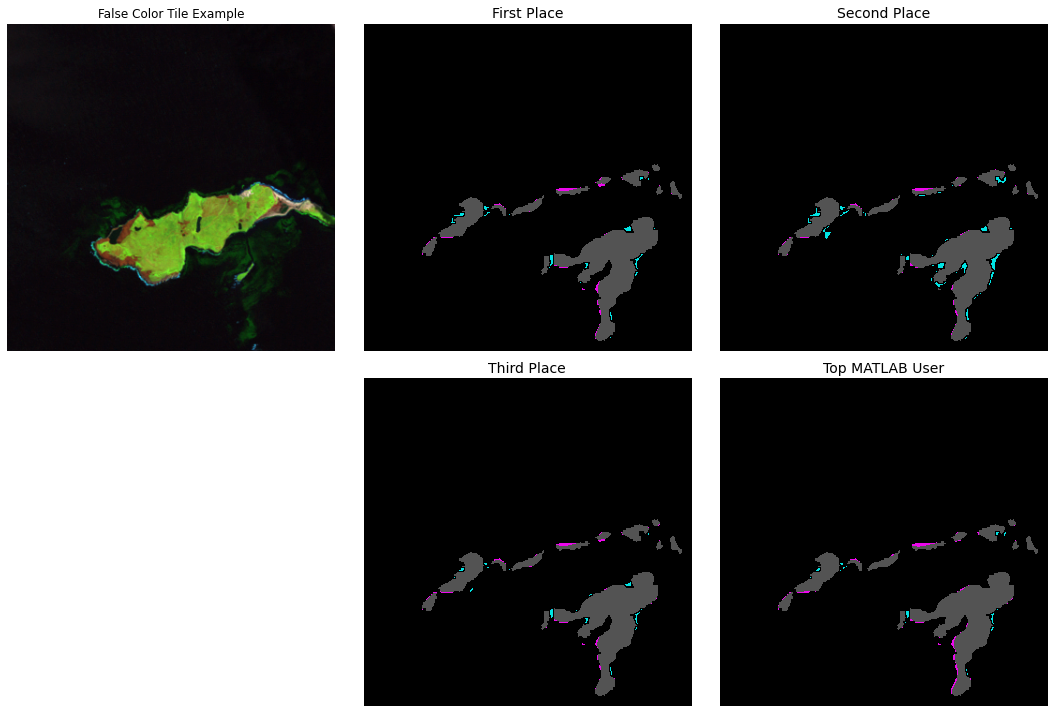
In this semantic segmentation challenge, the goal was to create an algorithm that predicts the presence or absence of kelp canopy using satellite imagery. The competitors were provided satellite images that were cropped to square 350 x 350 pixel "tiles" that correspond to patches of the coastal waters surrounding the Falkland Islands. For more information, you can read the competition's Problem Description.
To help participants get started, MathWorks published a benchmark solution that walks through how to train a basic semantic segmentation model using a SegNet network. The metric for this competition was Dice coefficient. It measures the similarity between two sets by considering their overlap relative to their individual sizes, providing a value between 0 (no overlap) and 1 (complete overlap). A higher Dice coefficient indicates better segmentation accuracy. In the case of binary segmentation, it is equivalent to F1-score.
Over the course of the competition, 671 participants battled it out and submitted a whopping 2,885 solutions! The top of the leaderboard remained fiercely contested throughout the competition, and the winners were ultimately able to achieve impressive results. The first place team secured the top spot with a Dice Coefficient of 0.7332. Close on their heels, second and third place scored 0.7318 and 0.7296, respectively. These results signify exciting advancements in the ability to accurately detect the presence and extent of kelp on a large scale.
The winners tested several creative strategies to build the best models. Below are a few interesting approaches common among the winners:
- Spectral indices: Generating features from the spectral indices proved crucial, especially those relying on the short-wavelength infrared (SWIR), near-infrared (NIR), and green bands.
- Image augmentations: The winners applied various augmentations to the training images, such as flips, rotations, cutmixes, and mosaics, which are commonly used techniques in computer vision tasks. Test-time augmentations were used with mixed results.
- Model architectures: All four winners created ensembles of deep learning models and relied on some combination of UNet, ConvNext, and SWIN architectures. Some teams also experimented with tree-based classifiers, either in their ensembles or to generate features.
Now, let's get to know our winners and how they created such successful kelp segmentation models! You can also dive into their open source solutions in the competition winners' repo.
Meet the winners
| Prize | Name |
|---|---|
| 1st place | Team Epoch IV |
| 2nd place | xultaeculcis |
| 3rd place | ouranos |
| Top MATLAB user | Team KELPAZKA |
Team Epoch IV


Place: 1st Place
Prize: $7,500
Hometown: Delft, Netherlands
Usernames and Social Media: EWitting (LI), hjdeheer (LI), jaspervanselm (LI), JeffLim (LI), tolgakopar (LI)
Background:
We are a group within Team Epoch, a student organization of the Technical University of Delft. We take a gap year to participate in AI competitions and projects, and organize and attend events. The team completely cycles every academic year, so the current members have been here for half a year. Five of us worked on Kelp Wanted.
What motivated you to compete in this challenge?
We look for AI competitions that contribute to the UN SDGs, and have a timeframe of 2~3 months. At the time of selecting competitions, this was the most attractive in terms of sustainability, image segmentation being a new type of challenge for this team, and having a topic that would be easy to explain and visualize at events.
Summary of approach:
For preprocessing, we first set all NaN values to zero. Then we engineered features like NDVI, NDWI, and ONIR, alongside derived features from NDVI such as edge detection and contrast enhancement. We also applied a slight Gaussian blur to the targets. Then we go through a feature selection step and fit a standard scalar.
In the modeling phase, XGBoost predictions serve as features for subsequent deep learning models. We ensemble models using three architectures: VGG-based UNET, Swin Transformer (SwinUNETR), and ConvNext. The parameters we used include 75 epochs, batch size of 16, layerwise learning rate decay, AdamW optimizer, and cosine learning rate decay scheduler with a 5-epoch warmup. Augmentations, such as rotations, flips, mosaic, and cutmix, are applied during training. We also used test-time augmentations of all flip and n*90 degree rotations. We employed a custom ensemble selection with weighted averaging on raw model logits. Finally, we fit a threshold based on maximizing the dice score on the validation set.

What are some other things you tried that didn’t necessarily make it into the final workflow?
Several attempted strategies failed to improve model performance. These included weighted dice loss, removing incorrectly labeled images, stacked ensembling, retraining the segmentation head, employing models like Prithvi and Torch Geo, using YOLO for segmentation, exploring loss functions other than dice loss, adjusting channel ranges, applying dithering, and experimenting with EfficientNet, as well as additional test-time augmentations like contrast and brightness adjustments.
If you were to continue working on this problem for the next year, what methods or techniques might you try in order to build on your work so far?
These are some interesting approaches that we have not tried, but we think they might lead to future improvements: upscaling of satellite images, using deep learning or classic techniques like kNN imputation/interpolation to fill in NaNs, trying different scalars (normalization, MinMaxScaler, etc.), tuning the threshold for submit to match kelp distribution on training data.
Michal Wierzbinski

Place: 2nd Place
Prize: $3,000
Hometown: Rabka-Zdroj (near the city of Cracow), Poland
Username: xultaeculcis
Social Media: GitHub, LinkedIn
Background:
ML Engineer specializing in building Deep Learning solutions for Geospatial industry in a cloud native fashion. Combining deep and practical understanding of technology, computer vision and AI with experience in big data architectures. A data geek by heart.
What motivated you to compete in this challenge?
My motivation to compete in the Kelp Wanted Competition stemmed from a confluence of professional interest and personal commitment to environmental sustainability. As an ML Engineer with a focus on geospatial analytics and deep learning, I am always on the lookout for challenges that push the boundaries of what's possible with AI in the realm of Earth observation and environmental monitoring. This competition represented a unique opportunity to apply my skills towards a cause that has profound implications for biodiversity, climate change mitigation, and the well-being of coastal communities worldwide.
Summary of approach:
In the end I managed to create two submissions, both employing an ensemble of models trained across all 10-fold cross-validation (CV) splits, achieving a private leaderboard (LB) score of 0.7318. I initially conducted detailed exploratory data analysis (EDA) to understand the dataset, identifying challenges like duplicate entries and missing Coordinate Reference System (CRS) information. To address duplicates, I generated embeddings for each image's DEM layer using a pre-trained ResNet network, grouping images with high cosine similarity. This de-duplication process led to a more robust CV split strategy, ensuring that the model was trained and validated on unique Area of Interest (AOI) groups. I established a baseline using a UNet architecture combined with a ResNet-50 encoder, trained on a 10-fold stratified CV split. This model used a combination of base spectral bands and single additional spectral index - the NDVI. Z-score normalization was applied to the input data. This baseline model achieved a public LB score of 0.6569.
The introduction of the Normalized Difference Vegetation Index (NDVI) and other spectral indices such as ATSAVI, AVI, CI, and more, enhanced the model's capabilities to distinguish between kelp and non-kelp regions. These indices, especially when coupled with strategy of reordering channels to align more closely with natural and scientific observations, significantly improved model performance. The decision to employ AdamW optimizer, accompanied by a carefully chosen weight decay and learning rate scheduler, further optimized the training process. The choice of a 32 batch size fully leveraged the computational capacity of the Tesla T4 GPUs, ensuring efficient use of resources.

The implementation of mixed-precision training and inference not only reduced model's memory footprint but also accelerated its computational speed, making the solution both effective and efficient. By adopting a weighted sampler with a tailored importance factor for each type of pixel, the models could focus more on significant areas, reducing the bias towards dominant classes. The UNet architecture, augmented with an EfficientNet-B5 encoder, proved to be the best combination for the task, striking a balance between accuracy and computational efficiency. Adjusting the decision threshold allowed me to fine-tune the model's sensitivity to kelp presence, which was crucial for achieving high evaluation scores.
Both of my top submissions were ensembles of models trained on diversified data splits, with specific attention to model weights and decision thresholds to optimize performance. TTA did not work for the public leaderboard. I opted to only optimize the individual model weights, soft labels usage and final decision threshold.
What are some other things you tried that didn’t necessarily make it into the final workflow?
Slicing Aided Hyper Inference or SAHI is a technique that helps overcome the problem with detecting and segmenting small objects in large images by utilizing inference on image slices and prediction merging. Because of this it is slower than running inference on full image but at the same time usually ends up having better performance, especially for smaller features. Best model trained on 128x128 crops with 320x320 resize and nearest interpolation resulted in public LB score of: 0.6848. As it turns out, the input time size of 350x350 is already too small for SAHI to shine. Sliced inference did not result in any meaningful bump in performance.
Another idea that did not work was training an XGBoost Classifier on all channels and spectral indices. The goal was not to use XGBoost to establish channel and spectral index importance, but rather completely replace the deep learning approach with a classical tree-based model. Unfortunately, the best models on public LB had score of 0.5125, which was way too low to try to optimize. Since predictions are done per pixel, TTA cannot be used. Optimizing the decision threshold did not improve the scores much. Even applying post-processing operations such as erosion or dilution would not bump the performance by 20 p.p.
If you were to continue working on this problem for the next year, what methods or techniques might you try in order to build on your work so far?
I'd definitely would try more models pre-trained on remote sensing data.
As well as transformer based models such as:
Would also like to leverage external data such as Sentinel-1 and 2 or Harmonized Landsat and Sentinel.
Ioannis Nasios

Place: 3rd Place
Prize: $1,500
Hometown: Athens, Greece
Username: Ouranos
Social Media: LinkedIn
Background:
I am a senior data scientist at Nodalpoint Systems in Athens, Greece. I am a geologist and an oceanographer by education turned to data science through online courses and by taking part in numerous machine learning competitions
What motivated you to compete in this challenge?
I consider myself as a machine learning engineer who enjoys taking part in various machine learning competitions. Furthermore, using machine learning for Earth Observation is a combination of my educational background and my professional occupation.
Summary of approach:
I blended models with different encoders and in various image sizes. Final models use the SWIR, NIR and Green channels. UNet models with mit_b1, mit_b2, mit_b3 and mit_b4 backbones, encoders from segmentation models pytorch library, as well as UperNet models with convnext_tiny and convenxt_base encoders from the transformers library were used. Image sizes of 512, 640, 768, 896 and 1024 were selected for the final models. As a post processing step, a 0.43 threshold turned probabilities to masks and a land-sea mask from last image channel was applied to remove predicted masks on land.
What are some other things you tried that didn’t necessarily make it into the final workflow?
Many other encoders. In particular, maxvit and hrnet encoders didn’t help the public LB score nor, I suspect, the private LB score, despite improving the local validation score. Also, training with functions other than soft dice loss didn’t seem to help in my experiments. Neither did color, mixup, cutmix, and a lot of other augmentations.
If you were to continue working on this problem for the next year, what methods or techniques might you try in order to build on your work so far?
As the dataset labels come from platform users' annotations, it contains many mislabeled images and this has passed on to trained models. For a real use case, a curated updated dataset followed by model retraining and parameters retuning should be used. If I continued working on this problem for the next year, I would prefer to work on a curated dataset for the models to be able to be used in a real project. But if I had to work on the exact same dataset, I would first reconsider my image and mask preprocessing, mask smoothing and boundary loss.
Team KELPAZKA
Place: Top MATLAB User
Prize: $3,000
Background:
My name is Azin Al Kajbaf. I am a postdoctoral research fellow at Johns Hopkins University and the National Institute of Standards and Technology (NIST). As a postdoctoral fellow, I am leveraging data science techniques and geospatial analysis to collaborate in projects to support community resilience planning through the development of methods and tools that evaluate the economic impacts of disruptive events.
My name is Kaveh Faraji. I am a Ph.D. candidate at the University of Maryland, and I work in the area of Disaster Resilience. The primary focus of my work is using geospatial analysis, statistical analysis, and machine learning in probabilistic risk assessment of critical infrastructure against natural hazards such as floods, sea level rise and hurricanes.
What motivated you to compete in this challenge?
We implement machine learning and deep learning methods in our research projects. We are interested to learn more about these approaches and their real-world application. Competing in these challenges allows us to gain experience with different machine learning and deep learning techniques that we can potentially employ in our research projects as well.
Summary of approach:
Our best scored solution is an ensemble of 19 U-Net convolutional neural network models. We used different U-Net structures with different number of layers, and several loss functions such as dice loss, focal loss and combination of these two. We also used multiple strategies for partitioning of the data.
What are some other things you tried that didn’t necessarily make it into the final workflow?
We started working on an XGBoost model, but due to time limitation, it did not end up in the final ensemble.
If you were to continue working on this problem for the next year, what methods or techniques might you try in order to build on your work so far?
If we were to continue working on this problem, we would have tried an ensemble of boosted trees and convolutional neural networks.
Thanks to all the participants and to our winners! Special thanks to MathWorks for supporting this challenge! Thanks also our partners at the Woods Hole Oceanographic Institution, the Byrnes Lab, and Zooniverse for providing their data and expertise! For more information on the winners, check out the winners' repo on GitHub.