

Welcome to the benchmark notebook for Mars Spectrometry 2: Gas Chromatography! The problem description for this challenge can be found here. The purpose of this notebook is to provide an example of how to use the data to create a basic benchmark model and to demonstrate how to submit your work.
Did Mars ever have livable environmental conditions? This is one of the key questions in the field of planetary science. NASA missions like the Curiosity and Perseverance rovers carry a rich array of scientific instruments to collect data that can help answer this question, including instruments that gather and analyze rock and soil samples. Using a method of chemical analysis called gas chromatography-mass spectrometry (GCMS), the samples can be analyzed for their chemical makeup, which can indicate whether the environment's conditions could have been amenable to life.
In this challenge, your goal is to build a model to automatically analyze GCMS data to detect the presence of nine families of chemical compounds related to understanding Mars' potential for past habitability. This challenge is a sequel to our first Mars Spectrometry challenge.
The winning techniques from this competition may be used to help analyze data from Mars, and potentially even inform future designs for planetary mission instruments performing in-situ analysis. In other words, one day your model might literally be out-of-this-world!
In this notebook, we'll cover:
- Exploratory data analysis
- Preprocessing
- Feature engineering
- Training a logistic regression model and a convolutional neural network
- Preparing a submission
Let's get started!
import itertools
from pathlib import Path
from pprint import pprint
import os
import shutil

from matplotlib import pyplot as plt, cm
import numpy as np
import pandas as pd
from pandas_path import path
from PIL import Image
from sklearn.dummy import DummyClassifier
from sklearn.preprocessing import minmax_scale
from sklearn.linear_model import LogisticRegression, LogisticRegressionCV
from sklearn.metrics import make_scorer, log_loss
from sklearn.model_selection import StratifiedKFold, cross_val_score
from tqdm import tqdm

import torch
import flash
from flash.image import ImageClassificationData, ImageClassifier
from flash.core.classification import ProbabilitiesOutput
from torch.utils.data import DataLoader
from pytorch_lightning import seed_everything

pd.set_option("max_colwidth", 80)
RANDOM_SEED = 42  # For reproducibility
tqdm.pandas()
Importing datasets
In this competition, there are three datasets:
- the training set, for which both features and labels are provided;
- the validation set, for which you will submit predictions, and your score will be displayed on the leaderboard while the competition is open
- the test set, for which you will also submit predictions, and your score will be used in determining the final rankings
This competition also has two phases: an initial development phase for the first half and a final training phase for the second half. In the second phase, the labels for the validation set will be released so that the validation set can be used as additional training data.
We will therefore perform light exploratory data analysis on the data available to us at the beginning of the competition - the features and labels for the training set. metadata.csv contains information about each sample included in the dataset, including whether it's a part of training, validation, or testing dataset.
PROJ_ROOT = Path.cwd().parent
DATA_PATH = PROJ_ROOT / "data/final/public/"
metadata = pd.read_csv(DATA_PATH / "metadata.csv", index_col="sample_id")
metadata.head()
train_files = metadata[metadata["split"] == "train"]["features_path"].to_dict()
val_files = metadata[metadata["split"] == "val"]["features_path"].to_dict()
test_files = metadata[metadata["split"] == "test"]["features_path"].to_dict()

print("Number of training samples: ", len(train_files))
print("Number of validation samples: ", len(val_files))
print("Number of testing samples: ", len(test_files))
Exploratory Data Analysis
The data for this competition is composed of gas chromatography mass spectra from laboratory instruments at NASA's Goddard Space Flight Center that are operated by the Sample Analysis at Mars (SAM) science team. A full description of the fields included in the data can be found in the problem description. The data for this challenge will likely feel familiar to participants in the first Mars Spectrometry challenge, as it is also mass spectrometry data.
First, let's visualize our mass spectra to see how these fields—time, mass, and intensity—relate to each other. Participants from the first Mars Spectrometry challenge may notice that we don't have a temperature column in the dataset. See the Problem Description for more on this. In this challenge, we'll be using time the way that temperature was used in the first challenge.
# Select sample IDs for five samples
sample_ids_ls = metadata.index.values[0:5]

# Import datasets for EDA
sample_data_dict = {}

for sample_id in sample_ids_ls:
    sample_data_dict[sample_id] = pd.read_csv(DATA_PATH / train_files[sample_id])
def plot_spectrogram(sample_df, sample_lab):
    # For visual clarity, we will round these intensity values to the nearest whole number and average the intensity.
    sample_df["mass"] = sample_df["mass"].round()
    sample_df = (
        sample_df.groupby(["time", "mass"])["intensity"].aggregate("mean").reset_index()
    )

    for m in sample_df["mass"].unique():
        plt.plot(
            sample_df[sample_df["mass"] == m]["time"],
            sample_df[sample_df["mass"] == m]["intensity"],
        )

    plt.title(sample_lab)
fig, ax = plt.subplots(1, 5, figsize=(15, 3), constrained_layout=True)
fig.suptitle("Samples")
fig.supxlabel("Time")
fig.supylabel("Intensity")

for i in range(0, 5):
    sample_lab = sample_ids_ls[i]
    sample_df = sample_data_dict[sample_lab]

    plt.subplot(1, 5, i + 1)
    plot_spectrogram(sample_df, sample_lab)

There are a few observations we can make from the above:
- There is a diversity in the time range of experiments (some are as short as 7 minutes, while others extend to nearly 40), and the intensity ranges differ as well.
- There are different m/z ion types that peak at different times. (Each colored line represents a distinct m/z value).
- For some samples, there are other ion types that are consistently present at low abundance levels. These are likely background abundances that are irrelevant. (In general, a spectrogram is useful for the peaks in abundances it shows at different times).
There is one more feature we have available in metadata that might be useful to our prediction task—derivatized. As described in the "Preprocessing Samples" portion of the problem description, some experiments are run after the sample is treated with a derivatization agent. Let's take a quick look at this feature.
metadata.derivatized.value_counts(dropna=False)
It seems that the derivatized is only ever 1 or NaN, indicating that we know which samples that are confirmed derivatized, but we do not know whether the remaining samples are definitely not derivatized. For additional information on how derivatization can affect a sample's mass spectrogram, see the problem description page.
Finally, let's also see what the distribution of compounds is in our training data.
train_labels = pd.read_csv(DATA_PATH / "train_labels.csv", index_col="sample_id")
target_cols = train_labels.columns
train_labels.head()
train_labels.aggregate("sum", axis=1).value_counts(normalize=True)
sumlabs = train_labels.aggregate("sum").sort_values()

plt.barh(sumlabs.index, sumlabs, align="center")
plt.ylabel("Compounds")
plt.xticks(rotation=45)
plt.xlabel("Count in training set")
plt.title("Compounds represented in training set")

We can make a few observations here:
- A large share (about 37 percent) of our samples do not have a positive label for any of the classes, and
- For some classes, such as chlorine-bearing compounds, other oxygen-bearing compounds, alcohols, and sulfur-bearing compounds, we have very few samples (less than 50).
Preprocessing
From the "Understanding GCMS Data" section of the project description page, we know that there are several preprocessing steps that will likely be helpful before working with the data. We'll demonstrate each step on a single sample to visualize the changes.
# Selecting a sample to demonstrate preprocessing steps

sample_df = pd.read_csv(
    DATA_PATH / metadata[metadata.split == "train"].features_path.iloc[0]
)
sample_df
Let's also calculate a few summary statistics on our dataset to have a sense of how these preprocessing steps will affect it.
# Calculate summary statistics for time and m/z values for training set


def get_time_mass_stats(fpath):
    df = pd.read_csv(DATA_PATH / fpath)

    time_min = df["time"].min()
    time_max = df["time"].max()
    time_range = time_max - time_min

    mass_min = df["mass"].min()
    mass_max = df["mass"].max()
    mass_range = mass_max - mass_min

    return time_min, time_max, time_range, mass_min, mass_max, mass_range
sample_paths_ls = metadata[metadata["split"] == "train"].features_path
training_stats_df = pd.DataFrame(sample_paths_ls)
training_stats_df.columns = ["fpath"]
(
    training_stats_df["time_min"],
    training_stats_df["time_max"],
    training_stats_df["time_range"],
    training_stats_df["mass_min"],
    training_stats_df["mass_max"],
    training_stats_df["mass_range"],
) = zip(*training_stats_df["fpath"].progress_apply(get_time_mass_stats))
training_stats_df.describe()
1. Standardizing which m/z values to include
As we can see in the summary statistics above and described in the problem description page, there is some heterogeneity in the m/z values measured for each sample. The range of m/z values being measured is not the same for every sample, and that most m/z values are fractional. In this section, we will make some basic simplifying assumptions to standardize which m/z values to include in our analysis. We have picked a threshold primarily to reduce dimensionality and make it easier for us to illustrate how to engineer features and train a model quickly, rather than one that is informed by the data or by domain knowledge. We encourage participants to devise their own approaches to preprocessing the data. In this example, we will discard any m/z values above 350, and we will round the fractional m/z values to their nearest integer and average their abundance values.
Additionally, as discussed on the problem description page, samples may have a high level of ions for m/z=4.0, which corresponds to helium carrier gas. The helium is not relevant to the composition of the sample, so we will also discard it as simplification. A more sophisticated analysis could potentially use it to understand how other ions compare to it relatively.
def drop_frac_and_He(df):
    """
    Rounds fractional m/z values, drops m/z values > 350, and drops carrier gas m/z

    Args:
        df: a dataframe representing a single sample, containing m/z values

    Returns:
        The dataframe without fractional m/z and carrier gas m/z
    """

    # rounds m/z fractional values
    df["rounded_mass"] = df["mass"].transform(round)

    # aggregates across rounded values
    df = df.groupby(["time", "rounded_mass"])["intensity"].aggregate("mean").reset_index()

    # drop m/z values greater than 350
    df = df[df["rounded_mass"] <= 350]

    # drop carrier gas
    df = df[df["rounded_mass"] != 4]

    return df
sample_df = drop_frac_and_He(sample_df)
2. Removing background ion presences
As discussed in the problem description, there will be background levels of ions in the measurements that aren't relevant to the analysis. While there are more complex and nuanced ways to remove the background noise, we will simply subtract the minimum abundance value. As mentioned in the project description, scientists may remove background noise more carefully. They may take an average of an area early in the experiment to subtract. Or, if the background noise varies over time, they may fit a function to it and subtract according to this function.
def remove_background_intensity(df):
    """
    Subtracts minimum abundance value

    Args:
        df: dataframe with 'mass' and 'intensity' columns

    Returns:
        dataframe with minimum abundance subtracted for all observations
    """

    df["intensity_minsub"] = df.groupby(["rounded_mass"])["intensity"].transform(
        lambda x: (x - x.min())
    )

    return df
# Intensity values before subtracting minimum
fig, ax = plt.subplots(1, 2, figsize=(15, 5))
fig.suptitle("Intensity values across temperature by m/z")
fig.supxlabel("Temperature")
fig.supylabel("Abundance levels")

plt.subplot(1, 2, 1)
for m in sample_df["rounded_mass"].unique():
    plt.plot(
        sample_df[sample_df["rounded_mass"] == m]["time"],
        sample_df[sample_df["rounded_mass"] == m]["intensity"],
    )

plt.title("Before subtracting minimum intensity")

# After subtracting minimum intensity value
sample_df = remove_background_intensity(sample_df)

plt.subplot(1, 2, 2)

for m in sample_df["rounded_mass"].unique():
    plt.plot(
        sample_df[sample_df["rounded_mass"] == m]["time"],
        sample_df[sample_df["rounded_mass"] == m]["intensity_minsub"],
    )
plt.title("After subtracting minimum intensity")

As we can see, simply subtracting the minimum intensity for this particular sample did not make a difference. There are likely better ways of accounting for noise in the data that are more sophisticated.
3. Convert abundances to relative abundances
Since the relative abundances of various ions are more informative than their absolute values, we normalize the abundance values from 0 to 1 within a single sample.
def scale_intensity(df):
    """
    Scale abundance from 0-1 according to the min and max values across entire sample

    Args:
        df: dataframe containing abundances and m/z

    Returns:
        dataframe with additional column of scaled abundances
    """

    df["int_minsub_scaled"] = minmax_scale(df["intensity_minsub"].astype(float))

    return df
Putting it all together
Finally, let's revisit what our samples look like after all of the preprocessing steps have been completed.
# Preprocess function
def preprocess_sample(df):
    df = drop_frac_and_He(df)
    df = remove_background_intensity(df)
    df = scale_intensity(df)
    return df
fig, ax = plt.subplots(1, 5, figsize=(15, 3), constrained_layout=True)
fig.suptitle("Commercial samples")
fig.supxlabel("Temperature")
fig.supylabel("Abundance")

for i in range(0, 5):
    sample_lab = sample_ids_ls[i]
    sample_df = sample_data_dict[sample_lab]
    sample_df = preprocess_sample(sample_df)

    plt.subplot(1, 5, i + 1)
    for m in sample_df["rounded_mass"].unique():
        plt.plot(
            sample_df[sample_df["rounded_mass"] == m]["time"],
            sample_df[sample_df["rounded_mass"] == m]["int_minsub_scaled"],
        )

    plt.title(sample_lab)

Feature engineering
When scientists analyze GCMS data, they look closely at the characteristics of peaks in ion abundances, such as the time at which they occur, the shape of the peaks including the height and area. For our analysis, we will engineer a simple set of features that try to capture some of these characteristics. We will discretize the overall time range into bins (since we do not have temperature information, time is the closest proxy), and calculate maximum relative intensity within that time bin for each m/z value. This is the same approach we used in our benchmark model for the previous challenge. Here, we will create 30-second time bins from 0 to 25 minutes. As with our selection of which m/z values to include, our choice of time bins and time range is meant to reduce dataset dimensionality in order to run this example quickly and without much computational expense, rather than being informed by the data or domain knowledge.
There are many ways to describe the shapes of these peaks with higher fidelity than the approach we demonstrate here. It will also be important to deal with complex cases such as peaks that overlap due to two different gas releases producing the same ions at around the same time. For inspiration, you may wish to consult the winners' code and write-ups from the previous challenge. We look forward to seeing what you all come up with in your own feature engineering.
# Create a series of time bins
timerange = pd.interval_range(start=0, end=25, freq=0.5)
timerange

# Make dataframe with rows that are combinations of all temperature bins and all m/z values
allcombs = list(itertools.product(timerange, [*range(0, 350)]))

allcombs_df = pd.DataFrame(allcombs, columns=["time_bin", "rounded_mass"])
allcombs_df.head()
We are expecting 350 m/z values * 50 time bins = 17,500 features to be generated per sample.
def int_per_timebin(df):
    """
    Transforms dataset to take the preprocessed max abundance for each
    time range for each m/z value

    Args:
        df: dataframe to transform

    Returns:
        transformed dataframe
    """

    # Bin times
    df["time_bin"] = pd.cut(df["time"], bins=timerange)

    # Combine with a list of all time bin-m/z value combinations
    df = pd.merge(allcombs_df, df, on=["time_bin", "rounded_mass"], how="left")

    # Aggregate to time bin level to find max
    df = df.groupby(["time_bin", "rounded_mass"]).max("int_minsub_scaled").reset_index()

    # Fill in 0 for intensity values without information
    df = df.replace(np.nan, 0)

    # Reshape so each row is a single sample
    df = df.pivot_table(
        columns=["rounded_mass", "time_bin"], values=["int_minsub_scaled"]
    )

    return df
# Assembling preprocessed and transformed training set

train_features_dict = {}
print("Total number of train files: ", len(train_files))

for i, (sample_id, filepath) in enumerate(tqdm(train_files.items())):
    # Load training sample
    temp = pd.read_csv(DATA_PATH / filepath)

    # Preprocessing training sample
    train_sample_pp = preprocess_sample(temp)

    # Feature engineering
    train_sample_fe = int_per_timebin(train_sample_pp).reset_index(drop=True)
    train_features_dict[sample_id] = train_sample_fe

train_features = pd.concat(
    train_features_dict, names=["sample_id", "dummy_index"]
).reset_index(level="dummy_index", drop=True)
train_features.head()
# Make sure that all sample IDs in features and labels are identical
assert train_features.index.equals(train_labels.index)
Perform modeling
This competition's task is a multi-label classification problem with 9 label classes—each observation can belong to any number of the label classes. One simple modeling approach for multi-label classification is "one vs. all", in which we create a binary classifier for each label class independently. Then, each binary classifier's predictions are simply concatenated together at the end for the overall prediction. For this benchmark, we will use logistic regression for each classifier as a first-pass modeling approach.
In order to have a reference point for our model, it can help to have a naive baseline. This challenge's metric is aggregated log-loss. Log-loss has the property that it is optimized by statistically calibrated predicted probabilities. Therefore, a good baseline model to use is to predict the proportion of each label class in the training set.
We will also use K-fold cross-validation to evaluate our model, rather than just a simple train-test split. K-fold cross-validation makes use of all of the data we have available for training and evaluation and is a useful technique for cases of having a relatively small amount of labeled data. When generating the cross-validation folds, we will also stratify according to class to make sure that there is even representation of each class for each fold. We will set a random seed in order to use the same cross-validation folds for both the dummy baseline model and the logistic regression model for an apples-to-apples comparison.
# Define stratified k-fold validation
skf = StratifiedKFold(n_splits=5, random_state=42, shuffle=True)

# Define log loss
log_loss_scorer = make_scorer(log_loss, needs_proba=True)
Baseline dummy classifier
# Check log loss score for baseline dummy model
def logloss_cross_val(clf, X, y):
    # Generate a score for each label class
    log_loss_cv = {}
    for col in y.columns:
        y_col = y[col]  # take one label at a time
        log_loss_cv[col] = np.mean(
            cross_val_score(clf, X.values, y_col, cv=skf, scoring=log_loss_scorer)
        )

    avg_log_loss = np.mean(list(log_loss_cv.values()))

    return log_loss_cv, avg_log_loss
# Dummy classifier
dummy_clf = DummyClassifier(strategy="prior")

print("Dummy model cross-validation average log-loss:")
dummy_logloss = logloss_cross_val(dummy_clf, train_features, train_labels[target_cols])
pprint(dummy_logloss[0])
print("\nAggregate log-loss")
dummy_logloss[1]
Now that we have a log-loss value from a very naive approach, we have a baseline against which to compare the performance of future approaches.
Logistic regression model
For our logistic regression models, we will also use lasso (a.k.a. L1) regularization, which will reduce the number of features used in the prediction. This will be helpful for the much greater number of features (17,500) than observations. More sophisticated dimensionality reduction techniques, such as principal component analysis (PCA), may be useful, but we will just stick with a simple approach for this benchmark. This is also the same as the benchmark model for the previous competition.
We've found that a regularization weight parameter of C=2 seems to work okay. To further tune this model, we would recommend using a cross-validated hyperparameter optimizer.
# Define Lasso model
logreg_clf = LogisticRegression(penalty="l1", solver="liblinear", C=2)
print("Logistic regression model cross-validation average log-loss:\n")
logreg_logloss = logloss_cross_val(logreg_clf, train_features, train_labels[target_cols])
pprint(logreg_logloss[0])
print("Aggregate log-loss")
logreg_logloss[1]
Training the model on all of the data
Now that we've used cross-validation to get an idea of our performance, we want to use all of the training data to train our model.
# Train logistic regression model with l1 regularization, where C = 2
def logreg_train(X_train, y_train):
    # Initialize dict to hold fitted models
    logreg_model_dict = {}

    # Split into binary classifier for each class
    for col in y_train.columns:
        y_train_col = y_train[col]  # Train on one class at a time

        # Output the trained model, bind this to a var, then use as input to prediction function
        clf = LogisticRegression(penalty="l1", solver="liblinear", C=2, random_state=42)

        logreg_model_dict[col] = clf.fit(X_train.values, y_train_col)  # Train

    return logreg_model_dict
fitted_logreg_dict = logreg_train(train_features, train_labels[target_cols])
# Create dict with both validation and test sample IDs and paths
all_test_files = val_files
all_test_files.update(test_files)
print("Total test files: ", len(all_test_files))
# Import submission format
submission_template_df = pd.read_csv(
    DATA_PATH / "submission_format.csv", index_col="sample_id"
)
compounds_order = submission_template_df.columns
sample_order = submission_template_df.index
def predict_for_sample(sample_id, fitted_model_dict):
    # Import sample
    temp_sample = pd.read_csv(DATA_PATH / all_test_files[sample_id])

    # Preprocess sample
    temp_sample = preprocess_sample(temp_sample)

    # Feature engineering on sample
    temp_sample = int_per_timebin(temp_sample)

    # Generate predictions for each class
    temp_sample_preds_dict = {}

    for compound in compounds_order:
        clf = fitted_model_dict[compound]
        temp_sample_preds_dict[compound] = clf.predict_proba(temp_sample.values)[:, 1][0]

    return temp_sample_preds_dict
# Dataframe to store logreg submissions in
final_submission_df = pd.DataFrame(
    [
        predict_for_sample(sample_id, fitted_logreg_dict)
        for sample_id in tqdm(sample_order)
    ],
    index=sample_order,
)
final_submission_df.head()
# Check that columns and rows are the same between final submission and submission format
assert final_submission_df.index.equals(submission_template_df.index)
assert final_submission_df.columns.equals(submission_template_df.columns)
The shape and layout of our prediction dataframe looks good! Each row is a unique sample and each column corresponds to a class. We will now generate a csv to submit.
final_submission_df.to_csv("benchmark_logreg_c2_submission.csv")
Upload submission
We can now head over to the competition submissions page to submit our predictions and see how we score! Click on "Make new submission" and upload your formatted prediction CSV file.
This is what we see when we submit our logistic regression-based predictions.

Our logistic regression model got a 0.2278 on the validation set. On the leaderboard, you can see that the naive model (named as "Training Set Prior Distributions") scored 0.2824. Not a bad start! Now, let's try one last approach.
Simple CNN model
In our previous Mars Spectrometry competition, the first-place winner used a neural network-based image classification approach to take home the prize. For this challenge, we will provide a simple example of how to use PyTorch Lightning Flash's image classification task with an out-of-the-box architecture (resnet18) to make predictions on the GCMS data. Neural networks have been used to analyze mass spectra in a variety of domains; audio spectrograms, current and voltage spectrograms, and even spectrograms that come from chemical analyses similar to our own have all been analyzed by scientists using neural networks.
The robustness of the first-place winner's model relied in part on much more refined feature engineering and modeling than we provide here; we leave it to you to improve upon this model. Feel free to check out the winners' repo for the previous Mars Spectrometry competition for inspiration.
Preprocessing
In order to train a simple neural network on this data, we will need to perform a few more preprocessing steps. While our previous approach relied on using tabular data as input, here we will use an image representation of the mass spectrogram that is based on the same features we used as input into our logistic regression model. As for the logistic regression model above, there are a variety of ways to engineer meaningful features, and we are simply using the features we have already generated for simplicity. There may be better ways to engineer features that yield better performance for image classification.
# We will turn each of the rows in train_features into an image

train_features
# Let's create a few directories to store these

IMG_OUTPUT_PATH = PROJ_ROOT / "data/interim/benchmark_testing"

TRAIN_IMG_PATH = IMG_OUTPUT_PATH / "train_features"
VAL_IMG_PATH = IMG_OUTPUT_PATH / "val_features"
TEST_IMG_PATH = IMG_OUTPUT_PATH / "test_features"
# Remove any existing train, val, or test features image directories and make new blank ones

for img_dir in (TRAIN_IMG_PATH, VAL_IMG_PATH, TEST_IMG_PATH):
    try:
        shutil.rmtree(img_dir)
    except FileNotFoundError:
        pass
    img_dir.mkdir(parents=True)
In order to represent our features in a way that makes it easy to visualize and provide as input to our image classification task, we will scale our 0-1 intensity values to 0-255 and replicate our features three times, one for each of the RGB channels.
def row2img(row, save=False):
    temp_arr = row.values.reshape(350, 50, 1)

    # Scale from 0-1 to 0-255, make uint8, squeeze to just two dims
    temp_arr = np.squeeze((temp_arr * 255).astype(np.uint8), axis=2)

    # Stack to 3 dims to mimic rgb image
    temp_arr = np.stack((temp_arr,) * 3, axis=-1)
    temp_img = Image.fromarray(temp_arr)

    # Save as image
    if save:
        outpath = IMG_OUTPUT_PATH / (
            str(metadata.loc[row.name]["features_path"])[0:-4] + ".jpeg"
        )
        temp_img.save(outpath)

    return temp_img
Let's observe what our features look like represented as an image!
train_sample_img = row2img(train_features.iloc[0])
plt.imshow(train_sample_img, aspect="auto")

There are a few points to note here:
Spectra vs. traditional images: While Lightning Flash has built-in pre-trained image classification model options, none of them were trained on images that quite looked like this. Transfer learning, which is the process of finetuning a model that has been trained on one corpus with another, can improve and speed up the training process. However, transfer learning works best when the original corpus the model was pre-trained on resembles the subsequent corpus.
Here, it is unclear that our spectrogram representations resemble the original ImageNet images that many of the pre-trained models included in Lightning Flash were trained on.
In this first pass, we will proceed with simply training a model using our own data, rather than finetuning a pretrained model. Pre-trained models may still be of use for spectrograms, but it may require more research and experimentation to understand how to tune them correctly. For example, some elements that may have been learned by a pre-trained image classification model, such as the position and orientation of lines, may also be useful in working with spectrograms. However some of the other elements that involve color, organic shapes, etc. may not be as useful. Selecting layers of pretrained models to "freeze" or "unfreeze" is an advanced strategy that is implementable using Lightning Flash, but we will forgo it here in favor of keeping our modeling approach simple.
Experiment time and image size: Second, this image representation reminds us that although not all experiments were the same length, the images for each representation will be. This means that the times for which there was no data collected will be represented as 0. This "padding" of the image is sufficient for this benchmark, but there may be other approaches.
# Apply to all training set images
train_features.apply(lambda x: row2img(x, True), axis=1)
# Assembling preprocessed and transformed training set

test_features_dict = {}
print("Total number of test files: ", len(all_test_files))

for i, (sample_id, filepath) in enumerate(tqdm(all_test_files.items())):
    # Load training sample
    temp = pd.read_csv(DATA_PATH / filepath)

    # Preprocessing training sample
    test_sample_pp = preprocess_sample(temp)

    # Feature engineering
    test_sample_fe = int_per_timebin(test_sample_pp).reset_index(drop=True)
    test_features_dict[sample_id] = test_sample_fe

test_features = pd.concat(
    test_features_dict, names=["sample_id", "dummy_index"]
).reset_index(level="dummy_index", drop=True)
# Apply to all training set images
test_features.apply(lambda x: row2img(x, True), axis=1)
# Store mean and std deviation for normalization later

train_mean = train_features.values.mean()
train_std = train_features.values.std()

print("Training set mean: ", train_mean)
print("Training set standard deviation: ", train_std)
Let's also include where to find each corresponding image in the labels file, and make sure that each label is an integer.
train_labels = pd.read_csv(DATA_PATH / "train_labels.csv", index_col="sample_id")

# Collect target class names to use later
target_cols = train_labels.columns.tolist()

# Make sure each label is an integer
train_labels = train_labels.astype(int)

# Include path to jpeg
train_labels["fpath_jpeg"] = TRAIN_IMG_PATH / (train_labels.index + ".jpeg")
train_labels.head()
# Check to make sure paths look ok

train_labels.iloc[0].fpath_jpeg
# Let's do the same for the test features, using the submission format file

submission_format = pd.read_csv(
    DATA_PATH / "submission_format.csv", index_col="sample_id"
)
submission_format["fpath_jpeg"] = submission_format.index.to_series().apply(
    lambda x: IMG_OUTPUT_PATH
    / (str(metadata.loc[x]["split"]) + "_features")
    / (str(x) + ".jpeg")
)
submission_format.iloc[0].fpath_jpeg
Modeling
Choosing which model to implement and how can be a complicated decision. Here, we have decided for simplicity to use resnet18, which is a deep learning architecture that has been used to success on some image classification tasks (a schema for resnet18 as well as its counterparts with more layers can be found here). The architecture is one of the built-in backbones that Lightning Flash offers. The winner for the previous Mars Spectrometry competition used resnet34.
# For reproducibility
seed_everything(42, workers=True)
A DataModule is a Lightning class that allows for easy ingestion of data by Lightning processing mechanisms. It includes information about where the inputs can be found, their labels, the size of the batch they should be ingested in, and how they should be transformed. Here, we are specifying that the dataframe train_labels contains the path to our input images (fpath_jpeg), and the labels that correspond to each sample (the list target_cols).
Normalization is a common preprocessing step when using a neural network for image classification. Since we are training on our own data rather than finetuning a pre-trained model, we will normalize to our own dataset's mean and standard deviation. Specifying the image size is also a common tranformation step, which you may leverage if your preprocessing results in images of varying sizes. It is also common when using pre-trained models to choose to normalize and resize one's images with the same parameters as those of the initial training set.
Finally, while it is typical practice to split the training set and use some of it for local evaluation, we are not doing so in this example in the interest of keeping this example computationally inexpensive.
# 1. Create DataModule

datamodule_train = ImageClassificationData.from_data_frame(
    "fpath_jpeg",
    target_cols,
    train_data_frame=train_labels,
    batch_size=1,
    transform_kwargs={
        "mean": (train_mean, train_mean, train_mean),
        "std": (train_std, train_std, train_std),
    },
)
As we build our ImageClassifier, we want to specify a few key parameters:
backbone: As mentioned earlier, resnet architectures are built-in backbone options for Lightning Flash, and all we need to do to use resnet18 is to setbackbone="resnet18".multi_label: The default ImageClassifier is for single-label data, so we must specify that our problem is a multi-label classification one.
# 2. Build the task

model_10 = ImageClassifier(
    backbone="resnet18",
    pretrained=False,
    labels=datamodule_train.labels,
    multi_label=datamodule_train.multi_label,
)
In order to retrieve the probabilities of every target class rather than the labels, we will attach ProbabilitiesOutput() to our model and specify that we are seeking multi-label classification. (The default value for the multi_label argument is False).
# 3. Attach the Output
model_10.output = ProbabilitiesOutput(multi_label=True)
When it comes to deciding on the number of epochs to train our model for, we want to account for the relatively small size of our dataset and a reasonable time constraint. 10 epochs seems like an appropriate starting point, as it is unlikely the model with overfit at this number, and we will be able to get predictions relatively quickly.
# 3. Create the trainer and train the model

trainer = flash.Trainer(max_epochs=10, gpus=torch.cuda.device_count())
trainer.fit(model_10, datamodule=datamodule_train)
# 4. Predict the targets

datamodule_predict = ImageClassificationData.from_data_frame(
    "fpath_jpeg",
    target_cols,
    predict_data_frame=submission_format,
    batch_size=1,
    transform_kwargs={
        "mean": (train_mean, train_mean, train_mean),
        "std": (train_std, train_std, train_std),
    },
)
predictions_10 = trainer.predict(
    model_10, datamodule=datamodule_predict, output=model_10.output
)

# 5. Save the model
trainer.save_checkpoint("image_class_resnet18_e10_nopre_trntfm.pt")
resnet18_e10_nopre_df = pd.DataFrame(
    np.array(predictions_10).squeeze(axis=1), index=sample_order, columns=target_cols
)
resnet18_e10_nopre_df.head()
Like for our logistic regression model, let's check to make sure that the row and column order match the submission format before submitting.
assert resnet18_e10_nopre_df.index.equals(submission_template_df.index)
assert resnet18_e10_nopre_df.columns.equals(submission_template_df.columns)
resnet18_e10_nopre_df.to_csv("benchmark_resnet18_e10_nopre_trntfm_submission.csv")
When we upload the submission to the platform, we will see this:

While the performance for this particular model isn't too impressive compared to our logistic regression (it performs about the same as the naive model), it might be a good starting point upon which to iterate. We look forward to seeing what you come up with!
GOOD LUCK!
We hope this benchmark solution provided a helpful framework for getting started. All three of the benchmark models have been added to the leaderboard for reference. Head over to the Mars Spectrometry 2: Gas Chromatography homepage for more details on the competition, and you can also check out the forum. We can't wait to see what you build!
Image of Curiosity courtesy of NASA/JPL-Caltech/MSSS