by
Isha Shah
The Challenge
Mass spectrometers are now, and will continue to be, a key instrument for missions searching for life and habitability on other planets. The results of this GCMS challenge could not only support NASA scientists to more quickly analyze data, but is also a proof-of-concept of the use of data science and machine learning techniques on complex GCMS data for future missions. Victoria Da Poian, NASA Goddard Space Flight Center Data Scientist & Engineer
Motivation
Did Mars ever have livable environmental conditions? NASA missions like the Curiosity and Perseverance rovers carry a rich array of instruments for collecting data that can contribute towards answering this question. One particularly powerful capability they have is collecting rock and soil samples and taking measurements that can be used to determine their chemical makeup. These chemical characteristics can indicate whether the environment had livable conditions in the past.
When scientists on Earth receive sample data from the rover, they must rapidly analyze them and make difficult inferences about the chemistry in order to prioritize the next operations and send those instructions back to the rover. In an ideal world, scientists would be to deploy sufficiently powerful methods onboard rovers to autonomously guide science operations and reduce reliance on a "ground-in-the-loop" control operations model.
The goal of the Mars Spectrometry 2: Gas Chromatography Challenge was to build a model to automatically analyze gas chromatography–mass spectrometry (GCMS) data collected for Mars exploration. Improving methods for analyzing planetary data can help scientists more quickly and effectively conduct mission operations and maximize scientific learnings.

The NASA Mars Curiosity rover.
In the previous DrivenData competition Mars Spectrometry: Detect Evidence for Past Habitability, competitors built models to predict the presence of ten different potential compounds in soil and rock samples using data collected using a chemical technique called evolved gas analysis (EGA). For this competition, participants used data collected using another method of chemical analysis that is used by the Curiosity rover's SAM instrument suite—gas chromatography–mass spectrometry (GCMS). Competitors used this GCMS data to predict the presence of nine different potential compounds.
For example, the first-place winner's model took the data on the left, which was from a sample that contained hydrocarbons, to generate the predictions on the right:
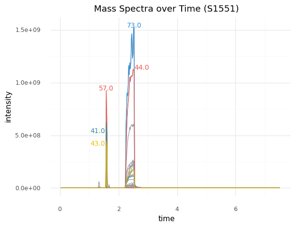
| aromatic | 0.008592 |
| hydrocarbon | 0.975277 |
| carboxylic_acid | 0.006051 |
| nitrogen_bearing_compound | 0.004336 |
| chlorine_bearing_compound | 0.000584 |
| sulfur_bearing_compound | 0.001165 |
| alcohol | 0.001052 |
| other_oxygen_bearing_compound | 0.002319 |
| mineral | 0.017754 |
| Note: compounds in blue were present in the sample. |
Results
Over the course of the competition, participants tested nearly 500 solutions and were able to contribute powerful models to the analysis of rock and soil samples using GCMS. To kick off the competition, DrivenData released a benchmark solution that demonstrated two approaches: (1) a simple logistic regression model and (2) a simple 2D CNN based on the first-place winner's solution from the initial Mars Spectrometry challenge.
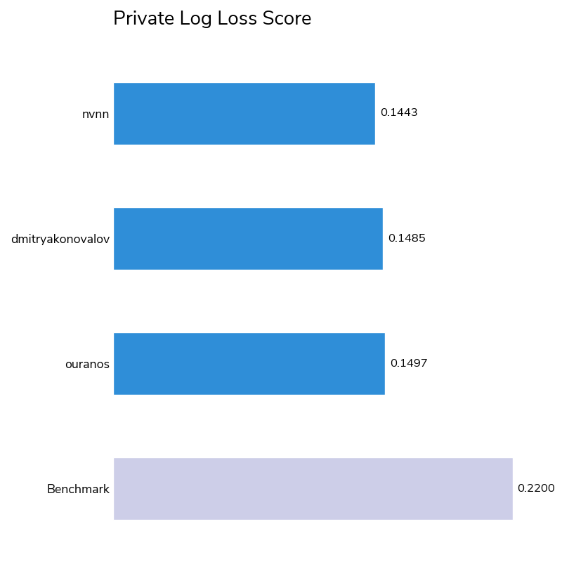
As with any research dataset like this one, initial algorithms may pick up on correlations that are incidental to the task. However, our winners were able to discern real trends driven by the chemical signatures of these compounds, as evidenced by their low aggregated log-loss scores (the metric for choosing the winners) and high micro-averaged average precision scores (a supplementary metric used to aid interpretability). 43 out of 80 competitors bested the logistic regression benchmark score of 0.22, with the winners achieving scores of 0.14 to 0.15.
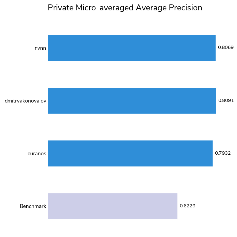
The winners also performed well on the micro-averaged average precision (a.k.a. area under precision–recall curve) metric. Average precision ranges from 0 to 1 (with 1 meaning perfect prediction) and measures how well models rank correct positive identifications with higher confidence than negative identifications. All three winners had average precision scores of at least 0.79, an impressive achievement given the smaller number and inherently noisier nature of GCMS samples compared to EGA samples and the absence of temperature data, an important feature that was present in the EGA mass spectrograms. Like the EGA data, the GCMS data used in this competition is unique and never previously used with machine learning.
This competition also featured a bonus prize, in which the top competitors were invited to submit a write-up of their approaches and the considerations that led them to their top-performing models. The write-ups were judged on four criteria:
- Performance: How well did the model perform on the test set?
- Interpretability: Does the modeling approach capture real underlying physical or chemical phenomena that would make it likely to generalize to future data?
- Innovation: Does the methodology involve any innovative or insightful analytical techniques that may generally benefit applications of gas chromatography–mass spectrometry for planetary science?
- Constructive discussion: Does discussion of how the methodology interacts with the provided data (e.g., results, modeling challenges) suggest concrete and actionable improvements to data collection for future research?
The judging panel was impressed by the quality and depth of all four bonus prize submissions. They each illustrated clear, context-aware approaches to predicting the compounds within GCMS samples and in many cases offered helpful visualizations to illuminate their models' inner workings. Ultimately, the judging panel chose the winning submission for its excellent constructive discussion of label noise, discussion about interactions between mass spectrometry data collection and machine learning, and interesting use of engineered features that capture peak information. All bonus prize write-ups are available alongside the winners' code in the winners' repo.
To build these high-performing and interpretable models, the winners brought a wide variety of creative strategies to this task! Below are a few common themes and approaches seen across solutions.
-
Feature engineering vs. neural network feature learning: The top performing solutions included deep learning models that used image or sequence representations of the data as inputs and feature engineering to capture the mass spectrograms. The first- and second-place winners used deep learning approaches and relied primarily on feature learning by their neural networks, while the third-place and bonus prize winners generated features to describe the mass spectrograms. The third-place winner combined both feature engineering and neural network feature learning.
-
1D vs. 2D deep learning: The first-place winner used a 1D CNN transformer whose output feeds into a 1D event detection model, and a 2D CNN whose output feeds into a 2D event detection model, while the second-place winner ensembled 13 different 2D CNNs with different preprocessing methods. The third-place winner also used two 2D CNN models with different architectures, but also combined them with two tree-based models (logistic regression and ridge classification). All winners who used deep learning fine-tuned pre-trained models.
-
Peak features vs. statistical features: The winners who generated features took different approaches to doing so: the third-place winner engineered statistical features across the entire sample (e.g., means and standard deviations of ion intensity per time interval), while the bonus prize winner engineered features that are commonly used in signal processing techniques, such as peak height and the derivative of ion intensities over time.
-
Ensembling: All of the winning solutions used some form of ensembling. Many trained multiple models with different types of preprocessing steps, model architectures, and deep learning model backbones. Some solutions also trained models on different subsets, or "folds", of the data. Ensembling, particularly with folds, can help avoid overfitting a model on the training data.
Now, let's get to know our winners and how they created such successful chemical analysis models! You can also dive into their open source solutions in the competition winners' repo.
Meet the winners
| Prize | Name |
|---|---|
| 1st place | Nghia NVN |
| 2nd place | Dmitry Konovalov |
| 3rd place | Ioannis Nasios |
| Bonus Prize | Dean Ninalga |
Nghia NVN
Place: 1st Place
Prize: $15,000
Hometown: Vietnam
Username: nvnn
Background:
I am a machine learning engineer, in my free time I participate in data science contests to learn new techniques and improve my data science skills.
What motivated you to compete in this challenge?
I want to gain new knowledge in this domain.
Summary of approach:
My solution is an ensemble of variants of 2 network architectures, both architectures are designed to detect the presence of targets in each time step and in the whole sample. The first architecture is based on 1D CNN-Transformer where each sample is transformed into a sequence of 1D arrays before feeding into a 1D Event Detection network. The second architecture is based on 2D CNN where 3 different preprocessing methods are applied to the sample to generate a 3 channel image-like representation, then this image-like representation is fed into a 2D Event Detection network.
What are some other things you tried that didn’t necessarily make it into the final workflow? LGB, Logistic regression, image classification approach.
If you were to continue working on this problem for the next year, what methods or techniques might you try in order to build on your work so far? The parameters are not carefully tuned yet. A hybrid approach that combines 1D and 2D representation should be considered as well.
Dmitry Konovalov

Place: 2nd Place
Prize: $7,500
Location: Townsville, Australia
Username: dmitryakonovalov
Background:
I am Dmitry Konovalov (PhD), currently working as a Senior Lecturer (Information Technology, Computer and Data Science) at the College of Science and Engineering of James Cook University, Townsville, Queensland, Australia. I teach computer programming, data science and software engineering courses. My research activities and publications are currently focused on solving computer vision and data science problems in marine biology and other applied/industry projects.
What motivated you to compete in this challenge?
I compete regularly in various competitions and am currently a Kaggle competitions expert (https://www.kaggle.com/dmitrykonovalov ). However, this is my first prize-winning finish on DrivenData. I mainly select competitions which are directly relevant to my research activities to learn and practice state-of-the-art solutions. In the predecessor Mars-1 competition, the first-place solution was entirely computer vision based and very elegant, which, together with the interesting dataset, inspired me to join this challenge.
Summary of approach:
- I followed the first-place solution of the previous Mars challenge by converting the mass spectrometry data into 2D images. Various CNN models and data-processing configurations were ensembled for the final 2nd-place winning submission.
- I experimented with different conversion configurations and found that the first 256 mass values (y-axis) were sufficient. For the time axis (x-axis), 192 time slots were selected as a reasonable baseline value, where larger values slowed down the CNN training.
- In this competition, time was only a proxy for temperature. Therefore, I only explored ideas where exact dependence on time values was not required. That led to two key ideas, which I think pushed my solution to the winning range.
- First, when training a CNN, the time dimension was randomly batch-wise resized on GPU within the 128-256 range of values. Then, at the inference phase, the corresponding TTA (test-time-augmentation) was done by averaging time sizes (5 steps of 32, centred at 192).
- The second win-contributing idea, I think, was creating a different classifier head, where only the time dimension of the CNN backbone 2D features was averaged (rather than both the mas and time dimensions) before the last fully connected liner layer.
- An extensive search of timm pre-trained models found HRNet-w64 to be particularly accurate for the considered 2D representation of data.
- Small but consistent improvement was gained by encoding the “derivatized” column as a 2-channel image and adding a trainable conversion layer before a CNN backbone.
- I was not able to achieve any consistent validation loss improvement by adding noise or smoothing/preprocessing original data at the training and/or inference stages. Hence, all training and inference were done with the original data converted to 2D images.
- For ensembling, averaging logits (inverted clipped sigmoids) rather than probabilities improved both validation and private LB results.
What are some other things you tried that didn’t necessarily make it into the final workflow?
Tried transformers, LSTM, adding noise, model and data dropouts.
If you were to continue working on this problem for the next year, what methods or techniques might you try in order to build on your work so far?
It seems that models’ diversity is the most important contributor to improving the competition metric. Therefore, the table-based methods (lightgbm etc), LSTM-like and 1D-transformers should be added.
Ioannis Nasios

Place: 3rd Place
Prize: $5,000
Hometown: Athens, Greece
Username: ouranos
Background:
I am a senior data scientist at Nodalpoint Systems in Athens, Greece. I am a geologist and an oceanographer by education turned to data science through online courses and by taking part in numerous machine learning competitions.
What motivated you to compete in this challenge?
I also competed in Mars 1 competition in Spring 2022. Both competitions combine my education in geology, my machine learning profession/skills and my personal interest for space. The fact that this was a NASA competition and results could someday be used for Mars exploration or space in general, was an extra motivation to me.
Summary of approach:
To increase variation three initial sets of data was created. Each model is trained using a different set of data. My final solution is an ensemble of four different type of models: logistic regression, ridge classification and simple neural networks, all trained with statistical features and pre-trained CNN trained with spectrogram type of data. One of the main difficulties in this competition was the small size of the dataset, with test data distribution being a little different from train one. Not to overfit required more attention and effort than usual. Ridge models are in principal the least overfitting models. Pretrained models also help not to overfit due to their starting point. Logistic regression only need one parameter to tune which is set constant during cross validation for all 9 classes for the same reason. Simple NN may overfit a little more than the other models and that’s why it is underweighted in final ensemble (all models are equal weighted, CV indicated an increased weight for simple NN = 2.5)
What are some other things you tried that didn’t necessarily make it into the final workflow?
Things that tried but didn’t make it to final ensemble:
- other models such as RNNs, transformers, tree models, tabnet and SVC,
- feature engineering
- sample mixing augmentation
- train NN with one label output at the time
If you were to continue working on this problem for the next year, what methods or techniques might you try in order to build on your work so far?
The difference between train and test distribution is not too large but it is possible and easy to overfit on train data. More data for training would be important for this task. Having more data could help make models that failed work and boost our results. New data are not always easy to be collected. Having to keep using the same datasets, I would stop my experiments with pseudolabels and I would work more with all other things that tried and didn’t work. Also, if training and inference speed is not an issue I would add more pretrained CNNs and probably add pytorch pretrained CNNs both for diversity and easier to access to more architectures.
Dean Ninalga

Place: Bonus prize
Prize: $2,500
Hometown: Toronto, Canada
Username: jackson5
Background:
Recently graduated in Mathematics & Statistics from the University of Toronto. I regularly participate in various online competitions.
What motivated you to compete in this challenge?
I was sitting on a few ideas that I knew could perform really well on time-series data based on my theoretical background and experience in other competitions. Moreover, I was motivated by the potential of helping the study of Mars and other interstellar bodies (in-situ or otherwise).
Summary of approach:
My solution is an ensemble of ten identical 3-layer Deep Neural Networks (or multilayer perceptrons) where each is trained using a loss with a Label Distribution Learning (LDL) component. LDL works well with data with label noise which I hypothesized existed in the data. I constructed the feature vectors using well-known peak detection techniques alongside n-difference features inspired by the derivative-producing algorithms seen in (older) works in analytical chemistry. Using these features validating ideas was hard since I observed a relatively high variance validation log-loss, even when averaging runs. This motivated me to use weight averaging which stabilized validation loss. Moreover, my best submissions use a weight-averaging algorithm I developed.
What are some other things you tried that didn’t necessarily make it into the final workflow?
Obviously, I tried a similar approach to the first Mars Spectrometry Challenge using large pre-trained convolutional neural nets early on. However, their performance was much worse compared to even low resource MLPs.
I also tried Auto-Sklearn which tries to find an optimal ensemble of models composed using any of the ML models found on the sklearn package. However, it could only perform well using an ensemble of MLPs.
If you were to continue working on this problem for the next year, what methods or techniques might you try in order to build on your work so far?
I definitely want to leverage other spectrometry datasets for gas chromatography or even liquid chromatography. More data is always a good thing.
Thanks to all the participants and to our winners! Special thanks to NASA for enabling this fascinating challenge and providing the data to make it possible! For more information on the winners, check out the winners' repo on GitHub.